Local Color Correction

Juan Gabriel Gomila Salas; Jose Luis Lisani

doi:10.5201/ipol.2011.gl_lcc

Juan Gabriel Gomila Salas, Jose Luis Lisani

→ BibTeX

@article{ipol.2011.gl_lcc,
    title   = {{Local Color Correction}},
    author  = {Gomila Salas, Juan Gabriel and Lisani, Jose Luis},
    journal = {{Image Processing On Line}},
    volume  = {1},
    year    = {2011},
    doi     = {10.5201/ipol.2011.gl_lcc},
}
% if your bibliography style doesn't support doi fields:
    note    = {\url{http://dx.doi.org/10.5201/ipol.2011.gl_lcc}}

published: 2011-09-27
reference: Juan Gabriel Gomila Salas, and Jose Luis Lisani, Local Color Correction, Image Processing On Line, 1 (2011). http://dx.doi.org/10.5201/ipol.2011.gl_lcc

Communicated by Jean-Michel Morel
Demo edited by Jose-Luis Lisani Roca

Juan Gabriel Gomila juan.gabriel@me.com Universitat de les Illes Balears (UIB)
José Luis Lisani Roca joseluis.lisani@uib.es Universitat de les Illes Balears (UIB)

Overview

In the context of this paper, by color correction techniques we refer to methods that increase the contrast of digital images.

When images are either too dark or too bright a classical gamma correction is enough to increase their dynamic range and improve their contrast.

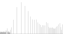
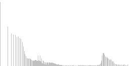
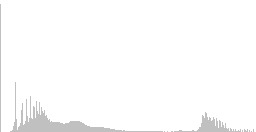
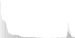
Figures 1 and 2 display two examples of contrast enhancement using gamma correction. In the first case a dark image is processed with γ=0.5, while in Fig. 2 γ=2.5 is used to process a bright image. The histograms of the resulting images show a clear increase of the dynamic range. In these examples is also shown that global histogram equalization doesn't perform well, since it increases excessively the dynamic range of the original images.

Figure 1. Effect of gamma correction with γ=0.5 on a dark image.

Figure 2. Effect of gamma correction with γ=2.5 on a bright image.

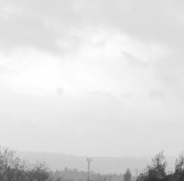
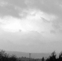
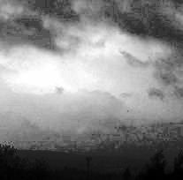
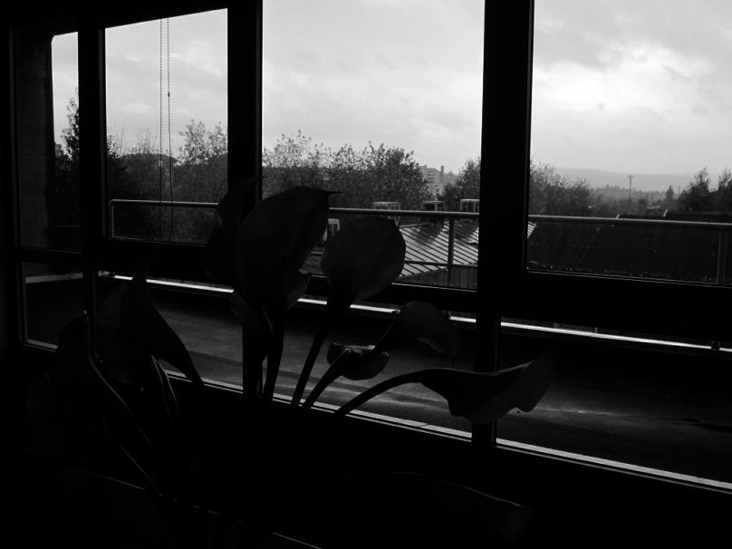
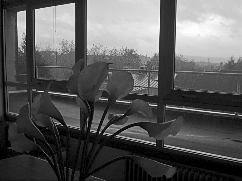
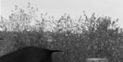
However, when images contain both dark and bright regions gamma correction techniques perform poorly (see Fig. 3). The reason is that gamma correction is a global technique. All pixels having a particular input intensity level are assigned the same output intensity, independent of the local context.

Figure 3. Gamma correction of an image with dark and bright regions with different values of γ.

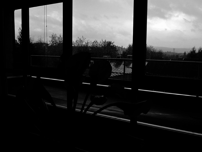
Results in Fig. 3 show that it is not possible to simultaneously improve the contrast of dark and bright regions using gamma correction. A compromise solution for choosing γ is to compute the mean grey level μ of the image and then use γ > 1 (implying attenuation of values) or γ < 1 (implying amplification of values) depending on whether μ is above 127.5 or below 127.5, respectively (we assume 8-bits images), according to the following formula, inspired by [1]:

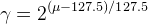$\gamma=2^{(\mu-127.5)/127.5}$ (*default* γ)

Other methods to automatically set the value of γ are explored in [3].

For the original image in Fig. 3, the default γ is 0.74, which gives almost the same result shown in Fig. 3 for γ=0.75.

In situations when shadows and highlights are present in the image, local techniques outperform global techniques. Local techniques can map one input value to many different possible output values, depending on the values of the neighboring pixels. This allows simultaneous shadow and highlight adjustment.

In this paper we present a local algorithm for contrast enhancement developed by N. Moroney at Hewlett-Packard Laboratories and presented at the IS&T/SID Eight Color Imaging Conference, in 2000 (US Patent 6,822,762, 2004). The algorithm uses a non-linear masking, is fast and does not require any manual parameter adjustments.

References

1. Moroney. Local Color Correction Using Non-Linear Masking IS&T/SID Eight Color Imaging Conference, pp. 108-111, 2000.
1. Moroney et al. "Local Color Correction" US Patent 6,822,762. November 23, 2004.
J.G. Gomila, J.L. Lisani. Gamma correction IPOL workshop, 2011
Pascal Getreuer. "colorspace"
Wikipedia: "HSI"
Wikipedia: "HSL and HSV"
Wikipedia: "YPbPr"

Online Demo

Try this algorithm on your own images with the online demo.

Algorithm (LCC algorithm)

Assume 8-bits RGB color images (R, G, B values in the range [0, 255]). The algorithm is computed in two steps:

A mask image is computed from the input image.
The input and mask images are combined to get the result.

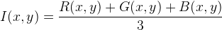
The mask image is computed from the intensity component of the color image, defined as the average of R, G and B values i.e. I=(R+G+B)/3. The use of intensity information avoids distortions of the chroma. The mask image is obtained by inverting and then blurring the intensity component of the input image:

Blurring is performed by using a Gaussian kernel of large radius, which guarantees that image contrast will not be excessively reduced along the edges (see discussion below). The resulting mask indicates which regions of the image will be lightened or darkened. For instance, a light region of the image will have a dark mask value, so it will be darkened.

The combination operation consists of a power function, where the exponent is computed using the mask value previously found. If the mask value is greater than 128, it will result in an exponent less than 1, while if the mask value is lower than 128, it will result in an exponent greater than 1. Moreover, if the mask value is precisely 128, the exponent will be 1, and it will have no effect on the input image. The operation is equivalent to a pixel-wise gamma correction and can be written as the following equation:

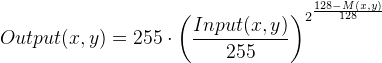$Output(x,y) = 255\cdot \left(\frac{Input(x,y)}{255} \right)^{2^{\frac{128-M(x,y)}{128}}}$ (1)

where, if (x,y) is a pixel coordinate of the image domain, Input(x,y) is the input image, M(x,y) is the computed mask and Output(x,y) is the output image.

If R, G, B are normalized in the range [0, 1], then the formulas can be simplified:

$I(x,y)=\frac{R(x,y)+G(x,y)+B(x,y)}{3}$ M'(x,y)=(Gaussian*I)(x,y)

$Output(x,y)=(Input(x,y))^{2^{(2M'(x,y)-1)}}$ (1b)

In the case of monochrome images Input(x, y) is the intensity component of the image. In [1] only results for monochrome images are shown.

For color images we have mainly two options:

Apply the algorithm channel by channel:
1. compute I and M' as in the formulas above
2. for (Input, Output) in {(R, new R), (G, new G), (B, new B)} apply formula (1b)

In the Results section (figures 6 and 7) it is shown that this option may lead to changes in chrominance.

Take a Luma+Chroma approach:
1. convert the input RGB image to a Luma+Chroma color representation,
2. apply LCC to the Luma component:
  
  $\text{new } Luma(x,y)=(Luma(x,y))^{2^{(2M'(x,y)-1)}}$
  
  (we assume Luma values in [0, 1]).
3. convert back to RGB using the new Luma and the original Chroma

In the second case, we have several possibilities, depending on the model for color representation that we choose. Since a discussion on which color model, if any, is better is beyond the goal of this paper we just decided to display the results of using three different models:

HSI. That is, Luma=I=(R+G+B)/3, Chroma=HS. In this case, preservation of chroma implies preservation of original R/G/B ratios.
HSL. That is, Luma=L, Chroma=HS.
YPbPr. That is, Luma=Y, Chroma=PbPr.

Refer to [4] for further information about color models and conversion formulas.

Comparisons of the various implementations of the algorithm are presented in the Results section.

Parameters of the algorithm.

The only free parameter of the algorithm is the radius (r) of the blurring filter used to obtain the mask image. As commented above, a certain amount of blurring is needed in order to avoid low contrasted edges. In particular, the author in [1] recommends to use a large radius, in such a way that image features can no longer be recognized. However, if the radius is too big the mask image will become uniform and the algorithm will reduce to a classical gamma correction. In the Results section we investigate the effect of the radius magnitude on various test images.

Implementation

Four versions of the local color correction (LCC) algorithm have been implemented (see previous section for details):

LCC-RGB: LCC algorithm applied channel by channel on the RGB input image.
LCC-HSI: Luma+Chroma approach using HSI color model.
LCC-HSL: Luma+Chroma approach using HSL color model.
LCC-YPbPr: Luma+Chroma approach using YPbPr color model.

In all the implementations, we have programmed the masking step by assuming that the original image has been extended by even symmetry.

Concerning the range of values for parameter r, we have decided to allow values between 0 (no blurring) to half the minimum dimension of the image. The use of larger radius implies almost uniform mask images. In such cases, we have decided to compute a global gamma correction with default γ:

$\gamma=2^{(\mu-127.5)/127.5}$ (2)

where μ is defined as follows:

average value of I=(R+G+B)/3, in LCC-RGB and LCC-HSI
average value of L, in LCC-HSL
average value of Y, in LCC-YPbPr

Source Code

An ANSI C implementation of the algorithm is provided: source code, documentation, online documentation

Basic compilation and usage instructions are included in the README.txt file. This code requires the libpng library.

Linux. You can install libpng with your package manager.
Mac OSX. You can get libpng from the Fink project.
Windows. Precompiled DLLs are available online for libpng.

Legal warning

Some of the files use algorithms possibly linked to the cited patent [2]. These files are made available for the exclusive aim of serving as scientific tool to verify the soundness and completeness of the algorithm description. Compilation, execution and redistribution of these files may violate exclusive patents rights in certain countries. The situation being different for every country and changing over time, it is your responsibility to determine which patent rights restrictions apply to you before you compile, use, modify, or redistribute these files.

The rest of files are distributed under GPL license.

Results

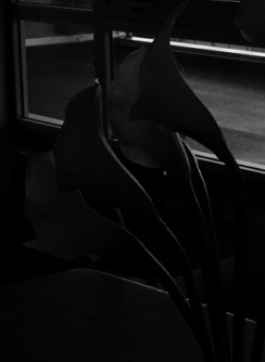
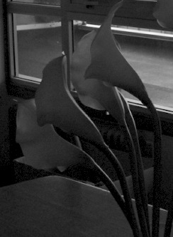
First, we start (Fig. 4) by testing the algorithm on the image displayed in Fig. 3, in order to check whether the algorithm is able to improve simultaneously the contrast of dark and bright regions.

The algorithm is run with different values of parameter r and the results are compared with a gamma correction with default γ (as defined by equation 2).

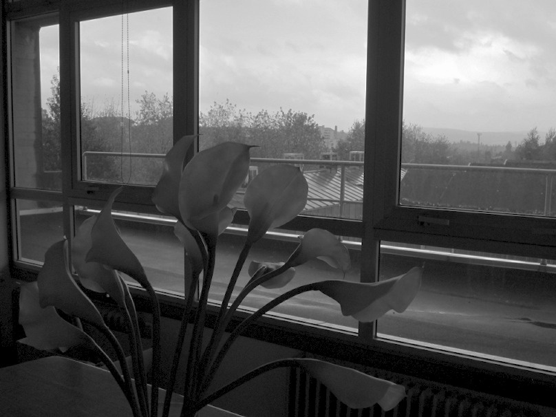
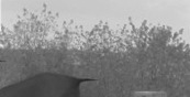
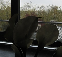
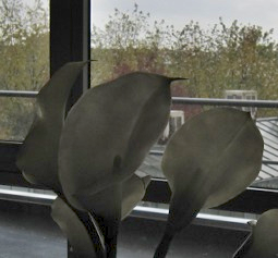
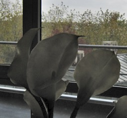
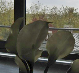
Figure 4. Local Color Correction of a monochrome image, with different values of the parameter. The result of global correction (gamma correction with *default* γ) is also displayed.

Results in Fig. 4 show that LCC outperforms classical gamma correction when shadows and highlights are simultaneously present at the scene. Moreover, the effects of variations of parameter r are appreciated when comparing different results: as r increases objects become sharper, their contrast with respect to surrounding objects increasing. Those effects are specially visible in the leafs of the trees (see detail in Fig. 5).

Figure 5. Detail of images in Fig. 4. Observe as contrast increases with *r*, although differences between *r=40* and *r=100* or *r=200* are small.

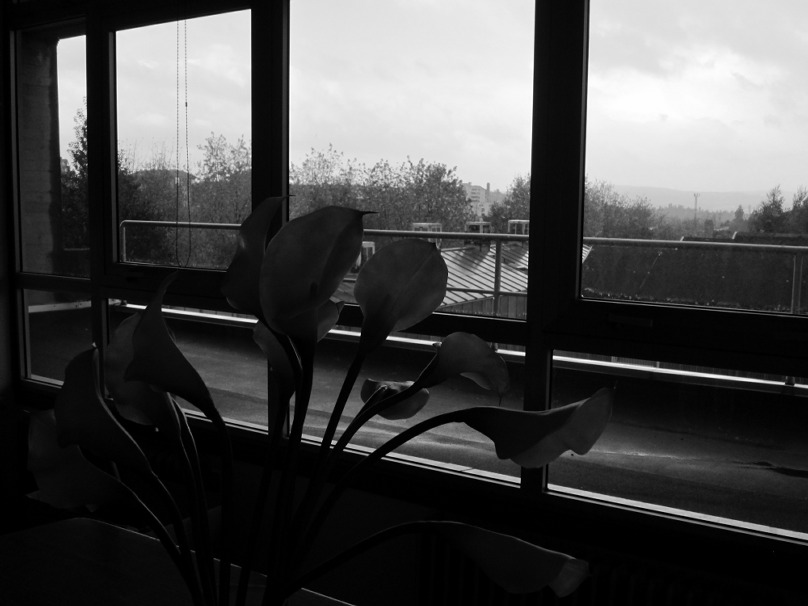
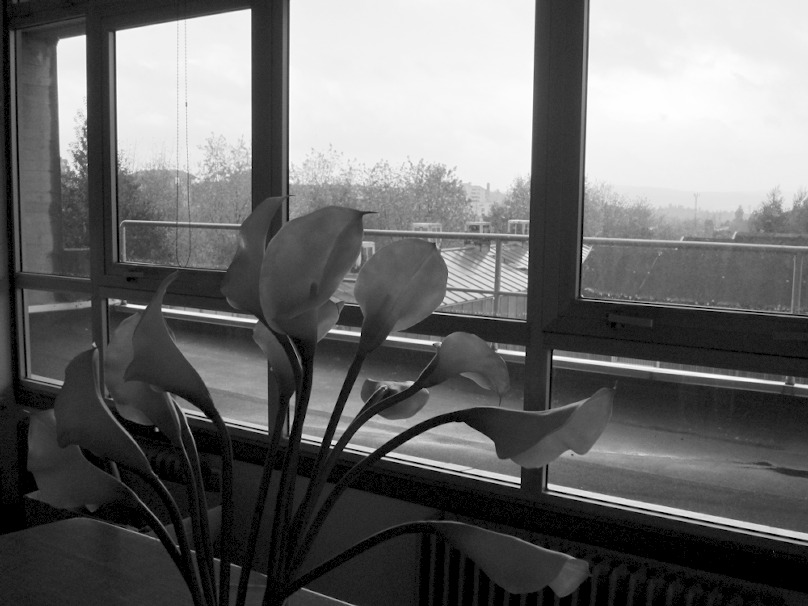
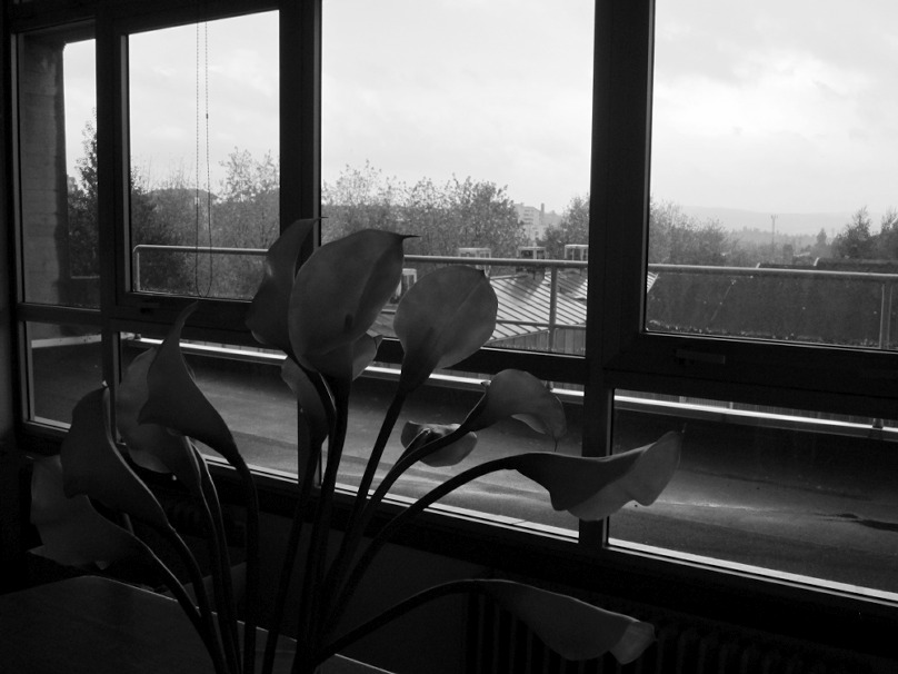
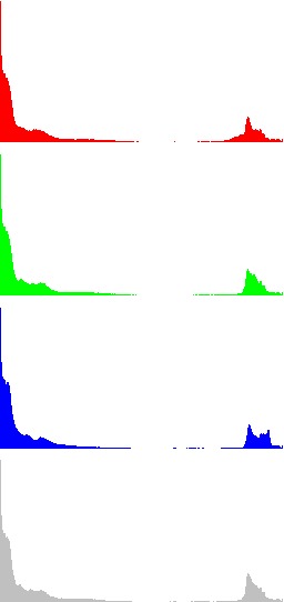
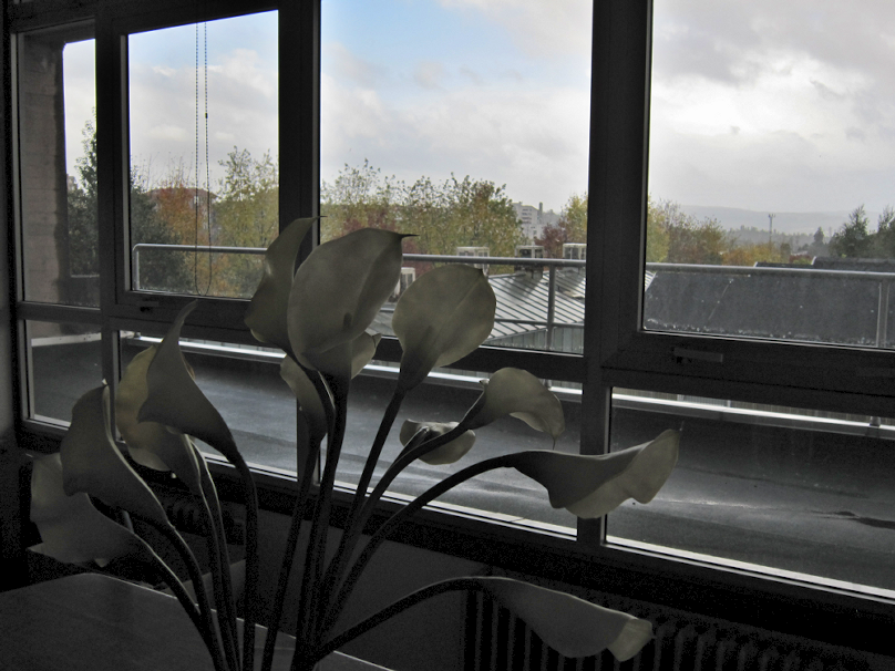
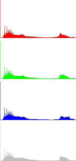
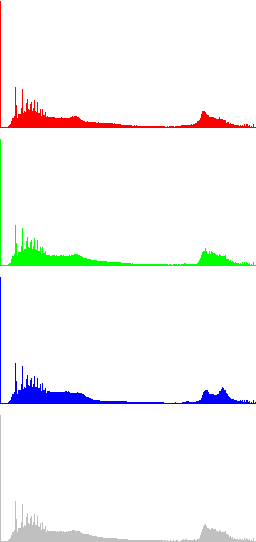
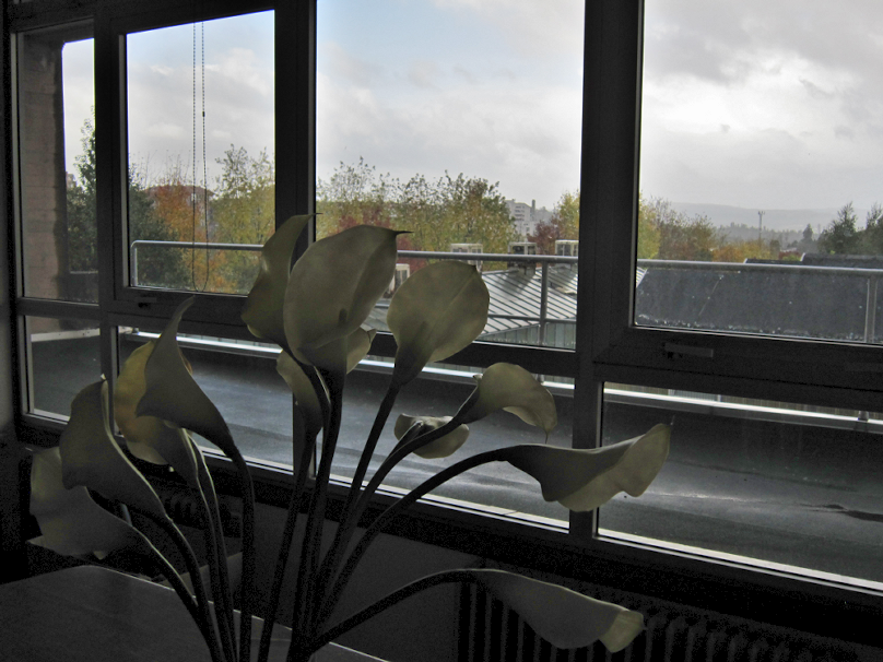
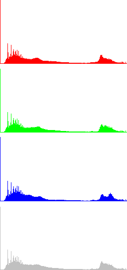
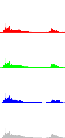
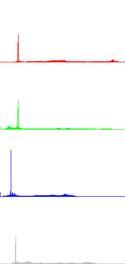
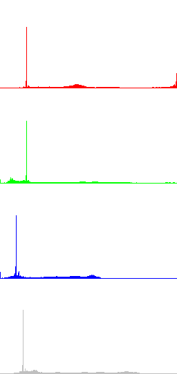
In the next Figures, color information is added to the images and the results of algorithms LCC-RGB, LCC-YPbPr, LCC_HSI and LCC-HSL are compared. We can also compare the results with the ones in Fig. 4, since a color version of the same original image is used in this test. Fig. 6 shows the results of the different versions of the algorithm for a fixed value of parameter r (r=40). The corresponding R, G, B and I histograms are also displayed. A detail of the image is displayed in Fig. 7, which permits to appreciate the differences between the results of the algorithms: LCC-HSI and LCC-HSL preserve the original chrominances (observe the yellowish colors of the flowers), while LCC-RGB and LCC-YPbPr alter this information (flowers are nearly white).

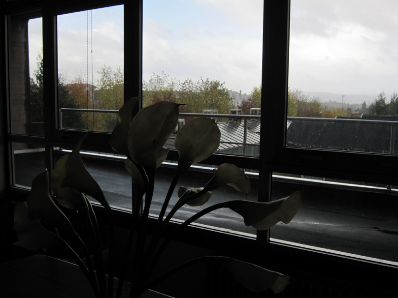
Figure 6. Local Color Correction of a color image, with a fixed value of the parameter (*r*=40). The results of algorithms LCC-RGB, LCC-YPbPr, LCC-HSI and LCC-HSL are displayed, together with the corresponding R, G, B and I histograms.

Figure 7. Detail of images in Fig. 6. Observe that LCC-HSI and LCC-HSL preserve the original yellowish colors of the flowers.

We conclude that, as expected, LCC-RGB does not preserve the chrominances of the original images. The same is true for LCC-YPbPr, even if it is based on a Luma+Chroma model. The versions of the algorithm based HSL and HSI do preserve these chrominances.

It must be remarked however that the HSI and HSL models perform poorly in dark regions, since the chrominance information in these regions is highly perturbed by noise. This can be appreciated in Fig. 8 where a false greenish color appears in the processed image.

Figure 8. These images illustrate the shortcomings of LCC-HSI and LCC-HSL models when applied on dark regions. In this example, a false greenish color appears in the processed image. LCC-RGB and LCC-YPbPr perform correctly. Results were obtained using *r*=40.

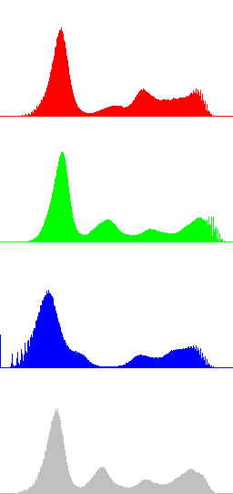
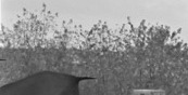
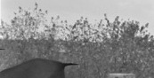
Figure 9 shows another example of the poor performance of LCC-HSI and LCC-HSL in dark regions. In this case the dark portion of the car is converted to very saturated red, which looks unnatural.

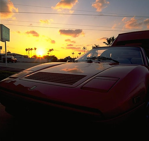
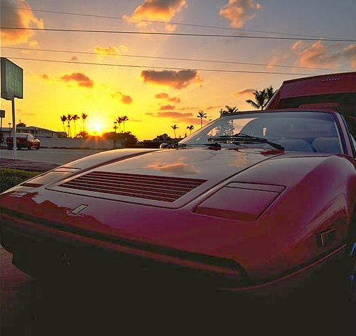
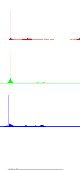
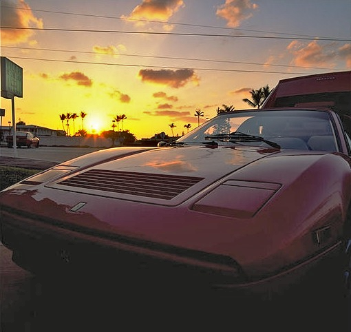
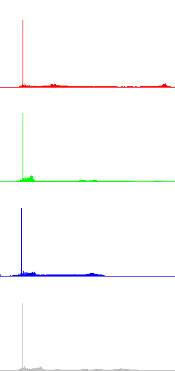
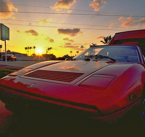
Figure 9. Using LCC-HSI and LCC-HSL dark red colors in the car become excessively saturated and they look unnatural. In this example LCC-YPbPr preserves correctly the original chrominances. Results were obtained using *r*=40.

The problem with HSI and HSL is that chrominance information is quite unreliable for almost-black colors (small perturbations of R, G and B produce very different values of H and S).

In particular, the problem with HSI is related to the R/G/B ratios having a singularity at black. Let I and I’ denote the original intensity and the LCC-corrected intensity, then the output colors are

$R'=(I'/I)R,\ G'=(I'/I)G,\ B=(I'/I)B$

If (R, G, B ) and its neighbors are almost black, then relative to intensities in [0, 1], the LCC-RGB output is approximately

$R'=\sqrt{R},\ G'=\sqrt{G},\ B=\sqrt{B}$

while the LCC-HSI output is approximately

$R'=R/\sqrt{I},\ G'=G/\sqrt{I},\ B=B/\sqrt{I}$

So the LCC-HSI output color (R', G', B') is more sensitive to small perturbations in an almost-black input color than the LCC-RGB output.

On the other hand, for an almost-black color, the output with this LCC-YPbPr procedure is approximately

$R' = \sqrt Y + 1.402Pr,\ \ G' = \sqrt Y - 0.344Pb - 0.713Pr,\ \ B' = \sqrt Y + 1.772Pb.$

where (Y,Pr,Pb) are a linear transformation of the input colors (R,G,B). So LCC-YPbPr’s sensitivity to perturbations is similar to LCC-RGB, so it works better than LCC-HSI for dark colors.